Contents
Electromagnetic fields are part of the spectrum ranging from static magnetic fields to high-intensity gamma rays. These fields are generated by the interaction between electric and magnetic field lines. EM fields are an important consideration while designing PCBs and require a field solver to predict their effect on the circuit board.
PCBs that support RF devices need to follow stringent design considerations to eliminate electromagnetic interference (EMI) and signal noise. While it is not possible to eliminate all EMI and noise issues, it is considered practical to minimize them while boosting electromagnetic compatibility (EMC). This is considered even more important when multiple boards need to be placed in close proximity during operation. Before we talk about field solvers, let us take a look at Maxwell’s equations to understand what field solvers do.
What are Maxwell’s equations?
Maxwell’s equations deal with electromagnetism and explain the phenomena with a set of 4 equations. A flow of electric current tends to generate a magnetic field. When this current flow varies with time, the magnetic field generates an electric field and vice versa. This is the phenomenon of electromagnetism. The equations are as follows:
Gauss’s law for electric fields
This law states that the electric flux through any closed surface is equivalent to the electric charge that is enclosed by the surface. This principle details the correlation between an electric charge and the electric field it generates.
![]()
E = Electric field in volts/m
ε0 = Permittivity of free space
ρ = Volume charge density in coulomb/m2
▽ = Nabla or del. It represents the vector operator (∂/∂x,∂/∂y,∂/∂z)
Gauss’s law for magnetism
The law states that the magnetic flux through any closed surface equals zero. This statement implies that magnetic field lines are continuous without an end or beginning. It eliminates the existence of magnetic monopoles.
![]()
B = Magnetic flux density in weber/m2
▽ = Nabla or del. It represents the vector operator (∂/∂x,∂/∂y,∂/∂z)

PCB Transmission Line eBook
5 Chapters - 20 Pages - 25 Minute ReadWhat's Inside:
- What is a PCB transmission line
- Signal speed and propagation delay
- Critical length, controlled impedance and rise/fall time
- Analyzing a PCB transmission line
Download Now
Faraday’s law
A changing magnetic field induces an electromotive force (EMF) leading to an electric field. The direction of the EMF that is induced opposes the change in the magnetic field.
![]()
E = Electric field in volts/m
t = Time in seconds (s)
B = Magnetic flux density in weber/m2
▽ = Nabla or del. It represents the vector operator (∂/∂x,∂/∂y,∂/∂z)
Ampère-Maxwell law
The Ampère-Maxwell law states that changing electric fields or moving charges generate magnetic fields.
![]()
Where,
E = Electric field in volts/m
J = Current density in amperes/m2
ε0 = Permittivity of free space
ρ = Volume charge density in coulomb/m2
t = Time in seconds (s)
B = Magnetic flux density in weber/m2
▽ = Nabla or del. It represents the vector operator (∂/∂x,∂/∂y,∂/∂z)
c = Light velocity in a vacuum

What are EM field solvers?
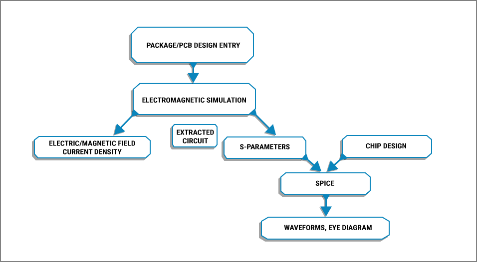
Electromagnetic field solvers are specific programs that solve Maxwell’s equations mentioned above to provide values for the magnetic flux and electric fields. Such field solvers are part of electronic design automation or EDA software used to design PCBs. Also, these solvers are required when high accuracy is needed for field parameters.
Electronic system designers use electromagnetic simulation to extract the parasitics of the board assembly and to calculate the electromagnetic fields for EMC and EMI.
Maxwell’s equations are solved by two methods:
- Use of a differential equation requiring discretization or meshing of the whole region in which the electromagnetic fields reside. This in turn is divided into the finite difference (FD) and finite element (FEM) methods.
- Integral equations are used for the discretization of the sources of the electromagnetic field.
The input to the field solver will be:
- The geometrical dimensions and material characteristics of the board or a board assembly
- The excitation at specified ports of the components such as pins or package leads
The resultant output will be the electric and magnetic fields generated by the board or board assembly. Such field parameters will make it easy to calculate current densities, electric potentials, S-parameters, impedances, and so on. The variables mentioned can be used to check signal and power integrity along with EMI.

The difference between 2D and 3D field solvers
2D field solvers compute electric fields in a cross-section along an X-Y plane. Hence this analysis can be applied only to planar structures and requires lesser computational effort than 3D field solvers.
In the case of 3D solvers, as the name suggests 3D geometries can be analyzed for fields for any frequency range and are known as full-wave 3D solvers.
The fields can be solved in the time or frequency domain. For time domain, you need to use finite difference time domain (FDTD) solvers. In the case of frequency domain, you need to employ the method of moments, namely finite element analysis and boundary element solvers (BEM).
Methods to solve EM fields
Electrical signals and therefore electromagnetic fields have both time and frequency domain representations. This involves the graphical representation of the signal strength, phase, and frequency. Here we will discuss such representations and their significance.
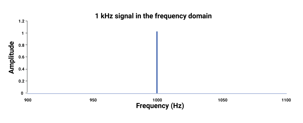
Frequency domain analysis
Signals can be represented by a magnitude and phase as a function of frequency and this is called frequency domain analysis. Frequency domain representations are particularly useful when analyzing linear systems. Also, system behavior and signal transformations are more convenient and intuitive when working in the frequency domain.
Need help in designing reliable PCBs? Our engineering team can help you with thermal management, stack-up design, and DFM analysis.
You can book a meeting with our experts or call us at +1 (800) 763-7503.

What are the basics of the finite element method (FEM)?
FEM is a mathematical technique to evaluate a process or structure by splitting it into various smaller units and systematically calculating the value of defined parameters for the units. Combining the individual values gives us the final result of the structure.
The mathematical equations behind FEM are applied to generate a simulation, also known as finite element analysis (FEA). This simulation is used to provide an analysis of required parameters such as structural stress or electromagnetic fields.
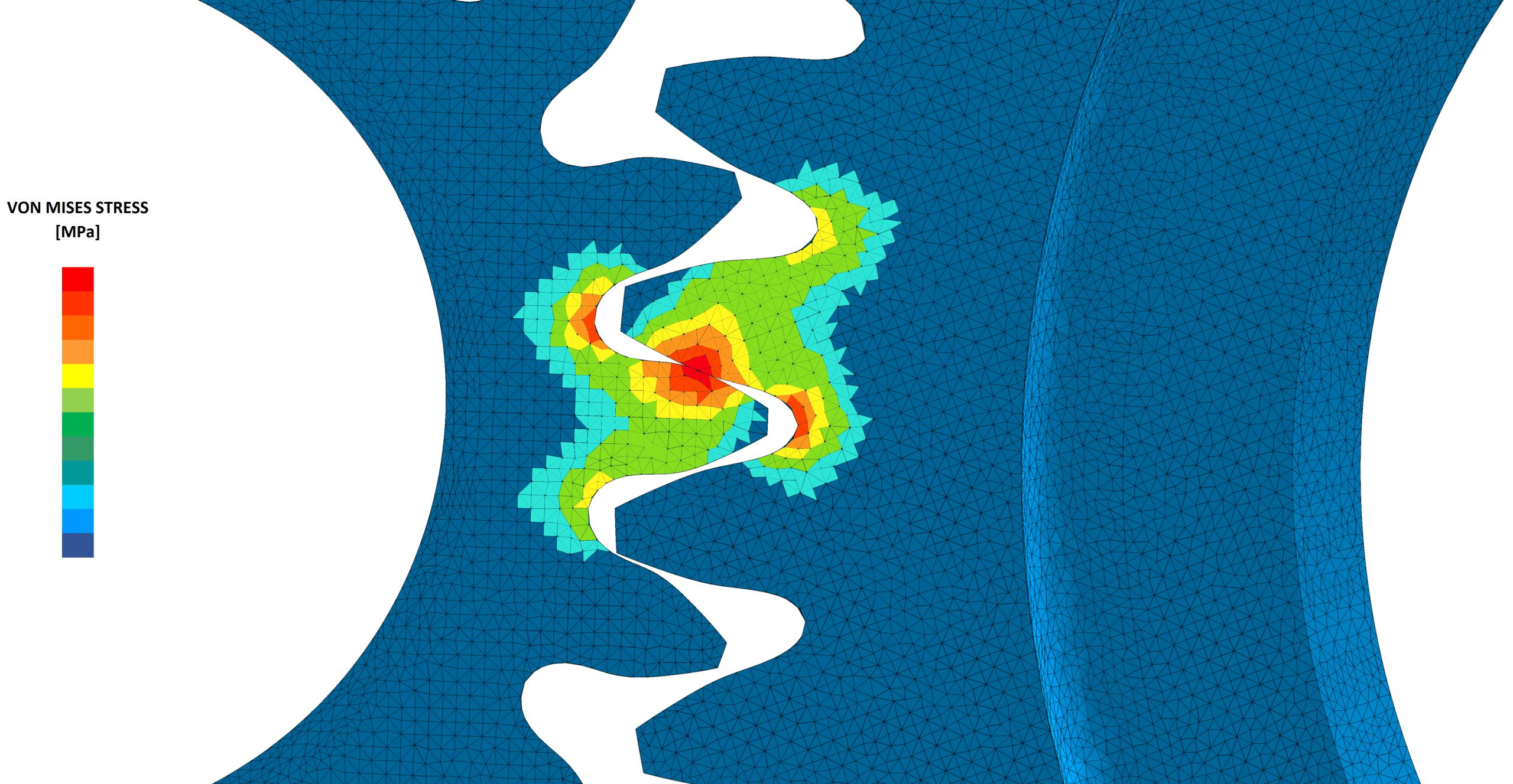
FEM is used to measure and solve EM fields using tools such as Hyperlynx by Siemens and 3D Solver Clarity by Cadence.
Given below is a table containing different methods to estimate electromagnetic compatibility:
| Analysis | Input data | Techniques | EMC estimation |
|---|---|---|---|
| Signal integrity analysis | Simplified driver- transmission line - receiver circuit | SPICE, IBIS, or user-defined models; fast circuit simulation, telegraph equations technique | Signal integrity verification |
| Spectrum analysis | Time domain PCB behavior; normalization constraints | Fourier transformation | Radiation |
| 2D EM field simulation | Technology parameters; circuit board geometry, transmission line parameters | Finite element method (FEM), boundary element method (BEM) | Transmission line parameters; reflection; 2D EM field current distribution |
| 3D EM field simulation | Virtual test environment | FEM, BEM; full wave simulation | 3D EM field, near and far field scan |

How do you use the boundary element method (BEM)?
The boundary element method (BEM) refers to a computational technique that involves solving linear partial differential equations which have been formulated as integral equations. This method is used for fluid mechanics, acoustics, and EMI calculations.
A partial differential equation is one that defines relations between the various partial derivatives of a multivariable function. The partial derivative of a multivariable function is its derivative with regard to one of those variables, while the other variables are held constant. In a total derivative, all variables are allowed to vary.
The integral equation can be considered as the exact solution to the governing partial differential equations. The boundary element method uses boundary conditions to define the integral equation with boundary values to get the solution at any given point within the region of interest.
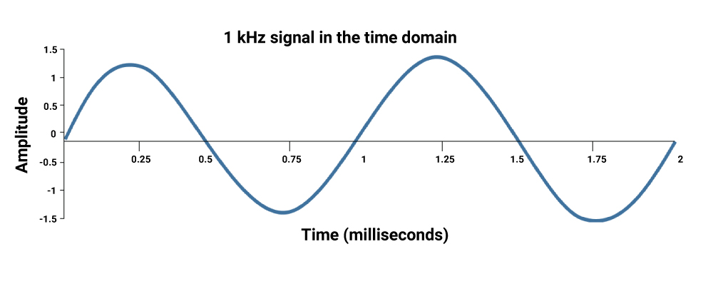
Time-domain analysis
In time domain, voltage or current is expressed as a function of time. Signal sources and interference are often defined in the time domain. Time-domain reflectometers (TDR) are used in such measurements.
What is finite difference time domain (FDTD) analysis?
Finite-difference time-domain (FDTD) analysis offers direct integration of Maxwell’s time-dependent equations. This is a volume-based method, hence it is exceedingly effective in modeling complex structures and media. FDTD being a time-domain technique implies that a single simulation results in a solution that measures the system response to a wide range of frequencies.
EM field solvers are critical to accurately estimate the EMC specific to PCB design and development. Hence PCB designers must be familiar with the use of such tools to ensure efficient board design. Let us know in the comments if you have any queries related to field solvers.

Signal Integrity eBook
6 Chapters - 53 Pages - 60 Minute ReadWhat's Inside:
- Impedance discontinuities
- Crosstalk
- Reflections, ringing, overshoot and undershoot
- Via stubs
Download Now